Financetoolkit

Next to that, I've also grouped the TQDM statements when using Ratios or Models. So instead of 5 bars, it displays just 2. Furthermore, I've extended the custom ratios functionality, see [here](https://www.jeroenbouma.com/projects/financetoolkit/custom-ratios).

| Strike Price | 2020-01-03 | 2020-01-04 | 2020-01-05 | 2020-01-06 | 2020-01-07 | 2020-01-08 | 2020-01-09 | 2020-01-10 | 2020-01-11 | 2020-01-12 | 2020-01-13 | 2020-01-14 | 2020-01-15 | 2020-01-16 | 2020-01-17 | 2020-01-18 | 2020-01-19 | 2020-01-20 | 2020-01-21 |
|---------------:|-------------:|-------------:|-------------:|-------------:|-------------:|-------------:|-------------:|-------------:|-------------:|-------------:|-------------:|-------------:|-------------:|-------------:|-------------:|-------------:|-------------:|-------------:|-------------:|
| 130 | -0 | -0 | -0 | -0 | -0 | -0 | -0 | -0 | -0.0001 | -0.0002 | -0.0004 | -0.0008 | -0.0015 | -0.0026 | -0.0041 | -0.0062 | -0.0089 | -0.0124 | -0.0167 |
| 135 | -0 | -0 | -0 | -0 | -0 | -0.0001 | -0.0003 | -0.001 | -0.0022 | -0.0043 | -0.0076 | -0.0122 | -0.0185 | -0.0265 | -0.0365 | -0.0486 | -0.0629 | -0.0794 | -0.0982 |
| 140 | -0 | -0 | -0 | -0.0003 | -0.0015 | -0.0045 | -0.0101 | -0.0192 | -0.0322 | -0.0493 | -0.0709 | -0.0968 | -0.1271 | -0.1616 | -0.2003 | -0.2429 | -0.2895 | -0.3397 | -0.3934 |
| 145 | -0 | -0.0004 | -0.0047 | -0.017 | -0.0396 | -0.0727 | -0.1156 | -0.1676 | -0.2277 | -0.295 | -0.3689 | -0.4486 | -0.5335 | -0.6233 | -0.7174 | -0.8154 | -0.917 | -1.022 | -1.13 |
| 150 | -0.0055 | -0.0485 | -0.1251 | -0.223 | -0.3353 | -0.4579 | -0.5883 | -0.7249 | -0.8666 | -1.0125 | -1.162 | -1.3145 | -1.4698 | -1.6275 | -1.7873 | -1.949 | -2.1125 | -2.2776 | -2.4442 |
| 155 | -0.2302 | -0.4512 | -0.671 | -0.8903 | -1.1094 | -1.3284 | -1.5474 | -1.7663 | -1.9853 | -2.2043 | -2.4234 | -2.6425 | -2.8617 | -3.081 | -3.3004 | -3.5198 | -3.7393 | -3.9589 | -4.1785 |
| 160 | -0.4343 | -0.8348 | -1.2016 | -1.5461 | -1.8754 | -2.1938 | -2.504 | -2.8078 | -3.1063 | -3.4006 | -3.6912 | -3.9787 | -4.2636 | -4.5461 | -4.8265 | -5.1051 | -5.382 | -5.6574 | -5.9314 |
| 165 | -0.452 | -0.9034 | -1.35 | -1.7871 | -2.2125 | -2.6264 | -3.0295 | -3.4229 | -3.8077 | -4.1848 | -4.5552 | -4.9194 | -5.2782 | -5.6322 | -5.9817 | -6.3272 | -6.6691 | -7.0076 | -7.3431 |
| 170 | -0.4657 | -0.9314 | -1.397 | -1.8618 | -2.3248 | -2.7846 | -3.2402 | -3.6907 | -4.1358 | -4.5753 | -5.0092 | -5.4376 | -5.8608 | -6.2788 | -6.6921 | -7.1007 | -7.5049 | -7.9051 | -8.3013 |

Furthermore, each module now has it's own dedicated Jupyter Notebook. Find all of them below or on my website [here](https://www.jeroenbouma.com/projects/financetoolkit).

- [Getting Started](https://www.jeroenbouma.com/projects/financetoolkit/getting-started)
- [Discovery Module](https://www.jeroenbouma.com/projects/financetoolkit/discovery-module)
- [Ratios Module](https://www.jeroenbouma.com/projects/financetoolkit/ratios-module)
- [Models Module](https://www.jeroenbouma.com/projects/financetoolkit/models-module)
- [Options Module](https://www.jeroenbouma.com/projects/financetoolkit/options-module)
- [Technicals Module](https://www.jeroenbouma.com/projects/financetoolkit/technicals-module)
- [Risk Module](https://www.jeroenbouma.com/projects/financetoolkit/risk-module)
- [Performance Module](https://www.jeroenbouma.com/projects/financetoolkit/performance-module)
- [Economics Module](https://www.jeroenbouma.com/projects/financetoolkit/economics-module)
- [External Datasets](https://www.jeroenbouma.com/projects/financetoolkit/external-datasets)

This release contains new Fixed Income metrics as part of the Economics module, these contain Option-Adjusted Spreads, Effective Yields, Total Returns and Yield to Worst. For example, see the Option-Adjusted Spread below (see documentation **[here](https://www.jeroenbouma.com/projects/financetoolkit/docs/economics#get_option_adjusted_spread)**):

<img width="410" alt="image" src="https://github.com/JerBouma/FinanceToolkit/assets/46355364/b645e60d-8ad0-4485-b23b-be1e7420eb7a">

The Option-Adjusted Spread (OAS) is the spread relative to a risk-free interest rate, usually measured in basis points (bp), that equates the theoretical present value of a series of uncertain cash flows to the market price of a fixed-income investment. The spread is added to the risk-free rate to compensate for the uncertainty of the cash flows. This is usually a better alternative than the usual Z-spread used to price derivatives.

Furthermore, northern-64bit (maintainer of [scikit-multilearn-ng](https://github.com/scikit-multilearn-ng/scikit-multilearn-ng)) introduced new AR and MA models that can be utilised with any type of time series. For more information, see https://github.com/JerBouma/FinanceToolkit/pull/117. northern-64bit actually introduced many more models in the Finance Toolkit as seen [here](https://github.com/JerBouma/FinanceToolkit/pulls?q=is%3Apr+author%3Anorthern-64bit).

Furthermore, I've introduced bug fixes solving 128 and 129.

This release includes the **Binomial Model**, a mathematical model for pricing both American as well as European options. The Binomial Model is a discrete-time model that calculates the price of an option by creating a riskless hedge portfolio that replicates the payoff of the option. The model is based on the assumption that the price of the underlying asset follows a binomial distribution. The Binomial Model is a simple and intuitive model that is widely used in practice. It is also the basis for more complex models. **See for an elaborate explanation the documentation as found [here](https://www.jeroenbouma.com/projects/financetoolkit/docs/options#get_binomial_model).**


For example, when using the following code:

python
from financetoolkit import Toolkit

companies = Toolkit(["AAPL", "MSFT"], api_key="FINANCIAL_MODELING_PREP_KEY")

companies.options.get_binomial_model(show_input_info=True)


It returns a large DataFrame with the binomial tree for each company and each strike price around the current price (as defined by the `start_date` parameter).

<img alt="image" src="https://github.com/JerBouma/FinanceToolkit/assets/46355364/59c14e7b-9c9a-4cda-9eff-e5e8e0ff928b">

The resulting output is a DataFrame containing the tickers, strike prices and movements as the index and the time to expiration as the columns. The movements index contains the number of up movements and the number of down movements. The output is the binomial tree displayed in a table. E.g. when using 10 time steps, the table for each strike price from each company will contain the actual binomial tree as also depicted in the image as seen below. Find the documentation [here](https://www.jeroenbouma.com/projects/financetoolkit/docs/options#get_binomial_model).

When selecting for example Apple at a Strike Price of 140 you will get the actual Binomial Tree depicted as a table, this represents the tree you see in the image at the top.

| Movement | 2024-02-02 | 2024-03-09 | 2024-04-15 | 2024-05-21 | 2024-06-27 | 2024-08-02 | 2024-09-08 | 2024-10-14 | 2024-11-20 | 2024-12-26 | 2025-02-01 |
|:-----------|-------------:|-------------:|-------------:|-------------:|-------------:|-------------:|-------------:|-------------:|-------------:|-------------:|-------------:|
| UUUUUUUUUU | 54.7747 | 69.9327 | 87.4757 | 107.31 | 129.344 | 153.573 | 180.122 | 209.208 | 241.069 | 275.965 | 314.18 |
| UUUUUUUUUD | nan | 39.9569 | 52.8423 | 68.2288 | 86.0206 | 106.037 | 128.14 | 152.365 | 178.911 | 207.994 | 239.852 |
| UUUUUUUUDD | nan | nan | 27.3011 | 37.7763 | 50.8718 | 66.5774 | 84.6651 | 104.825 | 126.925 | 151.146 | 177.689 |
| UUUUUUUDDD | nan | nan | nan | 16.9659 | 24.8886 | 35.4656 | 48.9066 | 65.0645 | 83.4462 | 103.602 | 125.698 |
| UUUUUUDDDD | nan | nan | nan | nan | 9.1158 | 14.4288 | 22.208 | 33.0259 | 47.083 | 63.8384 | 82.2161 |
| UUUUUDDDDD | nan | nan | nan | nan | nan | 3.8311 | 6.7007 | 11.4806 | 19.124 | 30.5822 | 45.85 |
| UUUUDDDDDD | nan | nan | nan | nan | nan | nan | 0.9669 | 1.9327 | 3.8631 | 7.722 | 15.4353 |
| UUUDDDDDDD | nan | nan | nan | nan | nan | nan | nan | 0 | 0 | 0 | 0 |
| UUDDDDDDDD | nan | nan | nan | nan | nan | nan | nan | nan | 0 | 0 | 0 |
| UDDDDDDDDD | nan | nan | nan | nan | nan | nan | nan | nan | nan | 0 | 0 |
| DDDDDDDDDD | nan | nan | nan | nan | nan | nan | nan | nan | nan | nan | 0 |

The model contains parameters to lengthen the time steps, change the risk-free rate and the dividend yield but more importantly, make it possible to calculate the price of both American and European options as well as Call and Put options. For example, let's calculate the price of a American Put option with a strike price of 140 for Apple again:

python
from financetoolkit import Toolkit

companies = Toolkit(["AAPL", "MSFT"], api_key="FINANCIAL_MODELING_PREP_KEY")

companies.options.get_binomial_model(
show_input_info=True,
put_option=True,
american_option=True,
timesteps=12,
risk_free_rate=0.01)


Which returns the Option valuations for an American Put Option.

| Movement | 2024-02-02 | 2024-03-03 | 2024-04-02 | 2024-05-03 | 2024-06-02 | 2024-07-03 | 2024-08-02 | 2024-09-01 | 2024-10-02 | 2024-11-01 | 2024-12-02 | 2025-01-01 | 2025-02-01 |
|:-------------|-------------:|-------------:|-------------:|-------------:|-------------:|-------------:|-------------:|-------------:|-------------:|-------------:|-------------:|-------------:|-------------:|
| UUUUUUUUUUUU | 2.3581 | 1.1115 | 0.4236 | 0.116 | 0.0171 | 0 | 0 | 0 | 0 | 0 | 0 | 0 | 0 |
| UUUUUUUUUUUD | nan | 3.7011 | 1.8524 | 0.7546 | 0.2225 | 0.0355 | 0 | 0 | 0 | 0 | 0 | 0 | 0 |
| UUUUUUUUUUDD | nan | nan | 5.6933 | 3.0346 | 1.3274 | 0.4238 | 0.0736 | 0 | 0 | 0 | 0 | 0 | 0 |
| UUUUUUUUUDDD | nan | nan | nan | 8.5588 | 4.8737 | 2.3002 | 0.8005 | 0.1529 | 0 | 0 | 0 | 0 | 0 |
| UUUUUUUUDDDD | nan | nan | nan | nan | 12.5322 | 7.6463 | 3.9148 | 1.4975 | 0.3173 | 0 | 0 | 0 | 0 |
| UUUUUUUDDDDD | nan | nan | nan | nan | nan | 17.8023 | 11.6676 | 6.518 | 2.7676 | 0.6586 | 0 | 0 | 0 |
| UUUUUUDDDDDD | nan | nan | nan | nan | nan | nan | 24.4233 | 17.2193 | 10.5575 | 5.0375 | 1.3671 | 0 | 0 |
| UUUUUDDDDDDD | nan | nan | nan | nan | nan | nan | nan | 32.2051 | 24.4052 | 16.5049 | 8.9884 | 2.8376 | 0 |
| UUUUDDDDDDDD | nan | nan | nan | nan | nan | nan | nan | nan | 40.6414 | 32.9347 | 24.6074 | 15.6102 | 5.89 |
| UUUDDDDDDDDD | nan | nan | nan | nan | nan | nan | nan | nan | nan | 48.9936 | 41.9389 | 34.3151 | 26.0772 |
| UUDDDDDDDDDD | nan | nan | nan | nan | nan | nan | nan | nan | nan | nan | 56.6615 | 50.2044 | 43.2257 |
| UDDDDDDDDDDD | nan | nan | nan | nan | nan | nan | nan | nan | nan | nan | nan | 63.702 | 57.7929 |
| DDDDDDDDDDDD | nan | nan | nan | nan | nan | nan | nan | nan | nan | nan | nan | nan | 70.1673 |

Under the hood of this model the stock prices are simulated based on up and down movements. These can be graphically depicted as a binomial tree and help in understanding the calculated option prices for each node in. More information about these stock price simulations can be found in the documentation [here](https://www.jeroenbouma.com/projects/financetoolkit/docs/options#get_stock_price_simulation) and as follows:

python
from financetoolkit import Toolkit

companies = Toolkit(["AAPL", "MSFT"], api_key="FINANCIAL_MODELING_PREP_KEY")

companies.options.get_stock_price_simulations(show_input_info=True, timesteps=10)


Which would return for Apple the following graph when plotted:


Given that the Finance Toolkit is modular, you do not have to use the Toolkit functionality directly and can also call each functionality of the model separately. For example, this shows the output of using the model directly, specifying each parameter yourself.

<img alt="image" src="https://github.com/JerBouma/FinanceToolkit/assets/46355364/b73d9bac-f4ee-44e3-863f-000572d7c21f">

This new release contains **intraday historical data** which makes it possible to calculate Risk, Performance and Technical metrics based on a 1 min, 5 min, 15 min, 30 min or 1 hour interval. For example, you can obtain the Capital Asset Pricing Model (CAPM) per model in which it calculates the beta for each hour.

<img src="https://github.com/JerBouma/FinanceToolkit/assets/46355364/395b98b9-5b7a-4f8a-8185-e0c5fe1f4b14" width="500px">

Or for example Williams %R on an hourly basis as follows:

<img width="567" alt="image" src="https://github.com/JerBouma/FinanceToolkit/assets/46355364/b7f953f3-6c40-498d-800d-4260dbeac600">

Next to that, I've done a lot of polishing. A user noticed that there were some issues with working with delisted companies. As Financial Modeling Prep allows you to get data on these companies whereas Yahoo Finance doesn't, I needed to make sure that the Finance Toolkit didn't attempt to query the Yahoo Finance and return an error. This has been resolved (all of these companies are delisted):


Furthermore, I've fixed small bugs, updated the documentation and more. All in all it should be a more pleasant experience!

v.1.8.0
It's time for another major release which consists of a full blown **Options menu** including all First, Second and Third Order Greeks such as Delta, Vega, Gamma, Theta and Ultima. Find the entire list of Greeks [here](https://github.com/JerBouma/FinanceToolkit?tab=readme-ov-file#options-and-greeks). Update your Finance Toolkit now with:

bash
pip install financetoolkit -U


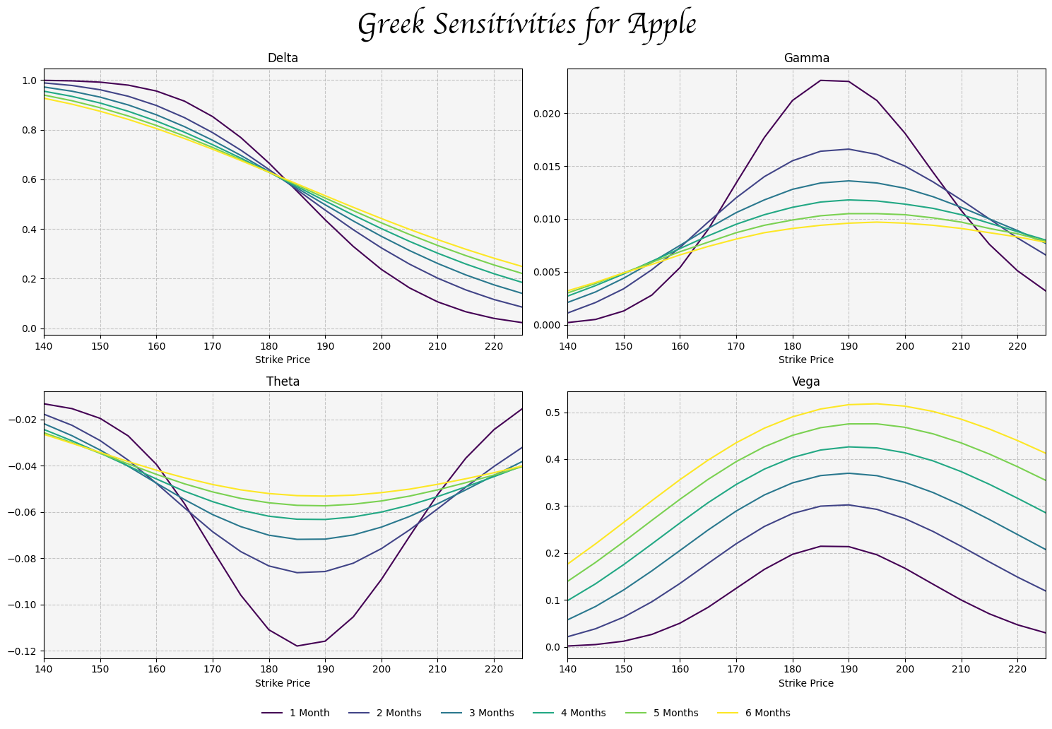
Based on the Black Scholes formula, it is now possible to get theoretical option prices and greeks for a range of stocks being able to plot charts such as the following:


For example, the following code gets you all Greeks for Tesla.

python
from financetoolkit import Toolkit

toolkit = Toolkit(["TSLA", "MU"], api_key="FINANCIAL_MODELING_PREP_KEY")

all_greeks = toolkit.options.collect_all_greeks(start_date='2024-01-03')

all_greeks.loc['TSLA', '2024-01-04']


Which returns (Stock Price: 238.45, Volatility: 55.4%, Dividend Yield: 0.0% and Risk Free Rate: 3.91%):

| Strike Price | Delta | Dual Delta | Vega | Theta | Rho | Epsilon | Lambda | Gamma | Dual Gamma | Vanna | Charm | Vomma | Vera | Veta | PD | Speed | Zomma | Color | Ultima |
|---------------:|--------:|-------------:|-------:|--------:|-------:|----------:|---------:|--------:|-------------:|--------:|---------:|--------:|--------:|----------:|-------:|--------:|--------:|--------:|---------:|
| 180 | 1 | -0.9999 | 0 | -0.0193 | 0.4931 | -0.6533 | 4.0782 | 0 | 0 | -0 | 0 | 0 | -0 | 0 | 0 | -0 | 0 | 0 | 0 |
| 185 | 1 | -0.9999 | 0 | -0.0198 | 0.5068 | -0.6533 | 4.4595 | 0 | 0 | -0 | 0 | 0 | -0 | 0 | 0 | -0 | 0 | 0 | 0 |
| 190 | 1 | -0.9999 | 0 | -0.0204 | 0.5205 | -0.6533 | 4.9195 | 0 | 0 | -0 | 0 | 0 | -0 | 0 | 0 | -0 | 0 | 0 | 0 |
| 195 | 1 | -0.9999 | 0 | -0.0209 | 0.5342 | -0.6533 | 5.4853 | 0 | 0 | -0 | 0 | 0 | -0 | 0 | 0 | -0 | 0 | 0 | 0 |
| 200 | 1 | -0.9999 | 0 | -0.0214 | 0.5479 | -0.6533 | 6.1981 | 0 | 0 | -0 | 0 | 0 | -0 | 0.0012 | 0 | -0 | 0 | 0 | 0 |
| 205 | 1 | -0.9999 | 0 | -0.022 | 0.5616 | -0.6533 | 7.1239 | 0 | 0 | -0 | 0.0004 | 0.0003 | -0 | 0.1071 | 0 | -0 | 0 | 0.0003 | 0.0001 |
| 210 | 1 | -0.9999 | 0 | -0.0226 | 0.5753 | -0.6533 | 8.3747 | 0 | 0 | -0.0002 | 0.0199 | 0.0108 | -0.0001 | 4.1973 | 0 | -0 | 0.0001 | 0.012 | 0.0032 |
| 215 | 0.9998 | -0.9997 | 0.0001 | -0.0252 | 0.5889 | -0.6532 | 10.1567 | 0.0001 | 0.0001 | -0.0041 | 0.414 | 0.1838 | -0.0027 | 72.9841 | 0.0001 | -0 | 0.002 | 0.198 | 0.0324 |
| 220 | 0.9974 | -0.9971 | 0.001 | -0.0512 | 0.601 | -0.6516 | 12.8704 | 0.0012 | 0.0014 | -0.04 | 4.0384 | 1.3972 | -0.0264 | 580.934 | 0.0014 | -0.0005 | 0.0141 | 1.4208 | 0.1193 |
| 225 | 0.9783 | -0.9767 | 0.0065 | -0.2027 | 0.6021 | -0.6391 | 17.2415 | 0.0075 | 0.0084 | -0.1863 | 18.7659 | 4.6975 | -0.1235 | 2158.08 | 0.0084 | -0.0022 | 0.0409 | 4.115 | 0.0867 |
| 230 | 0.8966 | -0.8912 | 0.0224 | -0.6437 | 0.5616 | -0.5857 | 24.2406 | 0.026 | 0.028 | -0.4003 | 40.2357 | 6.3078 | -0.2677 | 3809 | 0.028 | -0.0049 | 0.0261 | 2.5995 | -0.1644 |
| 235 | 0.6987 | -0.6885 | 0.0435 | -1.2217 | 0.4433 | -0.4565 | 34.5702 | 0.0504 | 0.0519 | -0.3092 | 30.7944 | 2.0098 | -0.2139 | 3626.75 | 0.0519 | -0.004 | -0.0676 | -6.8748 | -0.0997 |
| 240 | 0.4187 | -0.4074 | 0.0488 | -1.361 | 0.2679 | -0.2735 | 48.191 | 0.0565 | 0.0558 | 0.1652 | -17.2254 | 0.4231 | 0.0945 | 3408.71 | 0.0558 | 0.0014 | -0.0971 | -9.7985 | -0.0227 |
| 245 | 0.1798 | -0.1722 | 0.0327 | -0.911 | 0.1156 | -0.1174 | 64.4551 | 0.0379 | 0.0359 | 0.4473 | -45.5831 | 5.1158 | 0.2833 | 4082.47 | 0.0359 | 0.0049 | -0.0092 | -0.8794 | -0.1971 |
| 250 | 0.0534 | -0.0503 | 0.0136 | -0.3769 | 0.0344 | -0.0349 | 82.5525 | 0.0157 | 0.0143 | 0.322 | -32.7 | 6.4816 | 0.2066 | 3305.97 | 0.0143 | 0.0036 | 0.0467 | 4.7605 | -0.0412 |
| 255 | 0.0108 | -0.01 | 0.0036 | -0.0992 | 0.007 | -0.0071 | 101.798 | 0.0041 | 0.0036 | 0.12 | -12.1728 | 3.4389 | 0.0774 | 1510.91 | 0.0036 | 0.0014 | 0.0324 | 3.2868 | 0.1451 |
| 260 | 0.0015 | -0.0014 | 0.0006 | -0.017 | 0.001 | -0.001 | 121.702 | 0.0007 | 0.0006 | 0.0266 | -2.6915 | 0.9828 | 0.0172 | 404.445 | 0.0006 | 0.0003 | 0.0101 | 1.0246 | 0.1043 |
| 265 | 0.0001 | -0.0001 | 0.0001 | -0.002 | 0.0001 | -0.0001 | 141.935 | 0.0001 | 0.0001 | 0.0037 | -0.3769 | 0.1682 | 0.0024 | 66.8956 | 0.0001 | 0 | 0.0018 | 0.1826 | 0.031 |
| 270 | 0 | -0 | 0 | -0.0002 | 0 | -0 | 162.286 | 0 | 0 | 0.0003 | -0.0349 | 0.0183 | 0.0002 | 7.148 | 0 | 0 | 0.0002 | 0.0203 | 0.0051 |
| 275 | 0 | -0 | 0 | -0 | 0 | -0 | 182.618 | 0 | 0 | 0 | -0.0022 | 0.0013 | 0 | 0.5115 | 0 | 0 | 0 | 0.0015 | 0.0005 |
| 280 | 0 | -0 | 0 | -0 | 0 | -0 | 202.841 | 0 | 0 | 0 | -0.0001 | 0.0001 | 0 | 0.0253 | 0 | 0 | 0 | 0.0001 | 0 |
| 285 | 0 | -0 | 0 | -0 | 0 | -0 | 222.899 | 0 | 0 | 0 | -0 | 0 | 0 | 0.0009 | 0 | 0 | 0 | 0 | 0 |
| 290 | 0 | -0 | 0 | -0 | 0 | -0 | 242.753 | 0 | 0 | 0 | -0 | 0 | 0 | 0 | 0 | 0 | 0 | 0 | 0 |
| 295 | 0 | -0 | 0 | -0 | 0 | -0 | 262.382 | 0 | 0 | 0 | -0 | 0 | 0 | 0 | 0 | 0 | 0 | 0 | 0 |

Here, it automatically creates Strike Prices around the current stock price (or any price in the past if you change the start_date) parameter as well as plots forward for the time to expiration. Things that you can change with ease yourself if you like. For example:

python
from financetoolkit import Toolkit

toolkit = Toolkit(["MSFT", "ASML"], api_key="FINANCIAL_MODELING_PREP_KEY")

rho = toolkit.options.get_rho(
start_date="2020-01-02",
strike_price_range=0.15,
expiration_time_range=20,
put_option=True,
show_input_info=True
)

rho.loc['MSFT']


Which returns:

text
Based on the period 2013-01-22 to 2024-01-17 the following parameters were used:
Stock Price: ASML (291.79), Benchmark (305.06), MSFT (154.78)